I came across an common challenge in doing analytics on remote sensing data where we have missing time series data due to missed logs.

The use case in mind is predicting the spring thaw for Alaska's Arctic ice roads in the Tundra. These roads connect Arctic communities in the winter time allowing companies and people to trade and socialize. Each day having the ice road open is incredibly valuable, so knowing when the ice road is not safe to travel is critical.

The Data Generating Process

Here is a brief overview of the data-generating process

• Data loggers track both air temperature and ground temperature.
• There are other means to get air temperature where the ice road is generally located so we only deal with missing ground temperature data.
• Some data loggers are better at sending data than others.
• Data loggers are drilled into the ground. Ground/soil composition plays a part in the response to air time.
• We'll assume nothing else affects ground temperature (snow cover, sun radiation, etc.).

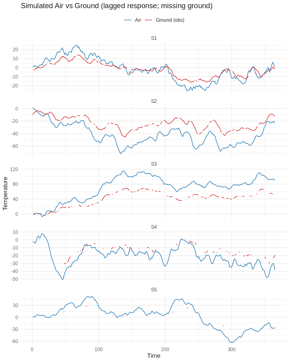
The data looks something like this, simulating data across five sensors:

The Model

We'll fit an heirarchical Vector Error Correction Model (VECM) with imputes for missing data. VECM accounts for long-run dynamics (the co-integration) and short-run dynamics.

The long-run dynamics are described in the co-integration equation:

$$G^*_{i,t} = (c_0 + c_i) + (\beta_0 + \beta_i)\,A_{i,t}.$$

Ground temperature $G$ at time $t$ from sensor $i$ has a long-run equilibrium with air $A_{i,t}$. $(c_0 + c_i)$ is the intercept of the relationship and $(\beta_0 + \beta_i$ is the marginal effect of a long-run change of air temperature to the ground temperature. The heirarchical relationship allows us to partially pool across the sensor locations.

The short-run dynamics are deviations from the long-run relationship where $z_{t-1,i} = G_{i,t-1} - (\beta_0 + \beta_i)A_{i,t-1} - (c_0 + c_i)$ are corrected over time:

$$\Delta G_{i,t} = \alpha_i\,z_{i,t-1} + \gamma_i\,\Delta A_{i,t} + \varepsilon_{i,t}.$$

Handling the missing data:

for the observed data we have:

$$y^{\text{obs}}_n \sim \mathcal{N}(\,G_{t_n,i_n},\,\sigma_{\text{obs}}\,)$$

for the missing data we have:

$$y^{\text{mis}}_m \sim \mathcal{N}(\,G_{\tau_m,j_m},\,\sigma_{\text{obs}}\,)$$

This approach allows us to impute data based on the DGP rather than just the ground temperature time series it self. This is especially important when there are a lot of missing data in the time series of interest and you would end up with huge credible intervals.

Running this in Stan, we can do the posterior imputation on the missing data:

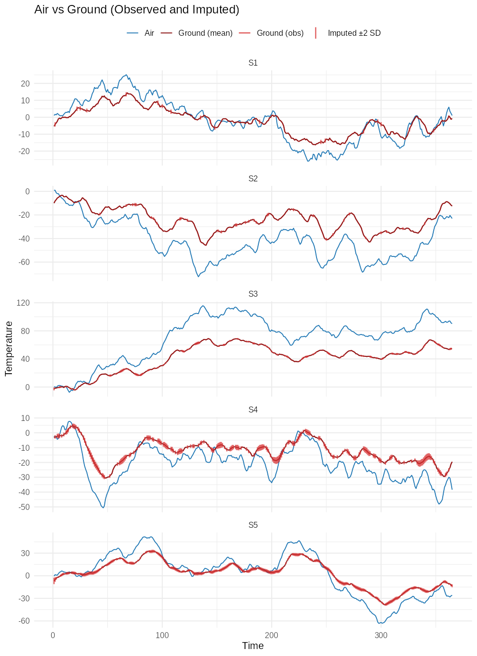Badda-bing. Badda-boom.

Extensions

The above is a simplification of the challenge in modeling but it's a good starting point for cases where:

• we need to relax assumptions for the case of spotty air temperature data. We could even have co-integration or partial-pooling across location air-temperature.
• Temperature variance varies across sensors / regions.
• We need to forecast using the best known air temperature forecast. We could also add posterior uncertainty for forecast error
• Add probability of unsafe conditions in the forecasts by ${i,t}$ (the Tundra threshold is often: -5C (27F) at 0.3 meters (1 foot))