Software in State-Space: modeling inter-dependence for "push to prod" decision-making

You ship a canary. It takes 10% of traffic, control keeps the rest. After a day you pull up p50 latency for both, treatment looks lower, you ship to 100%. That's the instinct most of us have, and it's wrong in two specific, fixable ways — and both come from testing metrics instead of testing the system.

This post walks through a small pipeline (code on GitHub) that fixes both, using an exact Kalman filter and a Gaussian copula. Neither is exotic once you see why they're there. The scenario: a canary rollout over a 500-step window. Control has been running the whole time and carries 90% of a spiky, bursty traffic process (diurnal cycle plus Poisson bursts). Treatment goes live partway through and only ever sees 10% of traffic. Three functions form a call chain — fetch_user -> get_recs -> render_html — that don't fail independently: a slow database cascades into everything downstream of it.

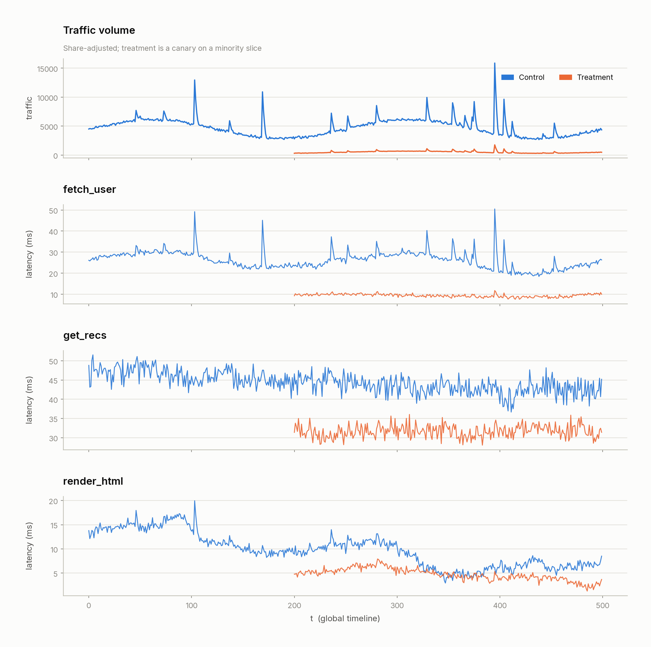
Stare at that for a second. Every latency spike lines up with a traffic spike. That's the first problem.

Problem 1: traffic is a confound, not noise

A canary isn't a controlled experiment in the classical sense — it doesn't get a random, equal-sized, time-matched slice of load. It gets whatever's left after control takes its share, at whatever time it happened to go live. So when you compare "treatment's average latency" to "control's average latency," you're not isolating the code change. You're also comparing how busy each arm happened to be, and busier periods raise latency for everyone regardless of code quality. A canary that looks fast might just be lightly loaded; a control that looks slow might have eaten every traffic spike in the window. Raw before/after numbers can't tell the two apart.

The fix is to explicitly model latency as a function of traffic, per function, per arm, and then compare what's left over once traffic is accounted for. Treat each function's latency as a small linear system whose coefficients drift over time:

$$\theta_t = \theta_{t-1} + w_t, \qquad w_t \sim \mathcal{N}(0, Q)$$ $$y_t = \alpha_t + \beta_t \cdot \text{traffic}_t + v_t, \qquad v_t \sim \mathcal{N}(0, \sigma_y^2)$$

where $\theta_t = [\alpha_t, \beta_t]$ is baseline latency and traffic-sensitivity at time $t$. This is a linear-Gaussian state-space model (a dynamic linear model), which means the online filtering distribution $P(\theta_t \mid y_{1:t})$ — a mean and its exact uncertainty, at every timestep, using only past data — has a closed form: the Kalman filter¹². No sampler, no convergence diagnostics, deterministic given the seed, and it runs in seconds.

It's worth naming the alternative, because it's the default a lot of us reach for: sample the trajectory with MCMC (e.g. PyMC's GaussianRandomWalk + NUTS). On the low-traffic canary arm, that produces divergences, max-treedepth warnings, and r-hat as high as 1.4 — the classic symptoms of asking an approximate sampler to do a job that already has an exact solution. If your model is truly linear-Gaussian, reach for the Kalman filter first and save MCMC for where you actually need it.

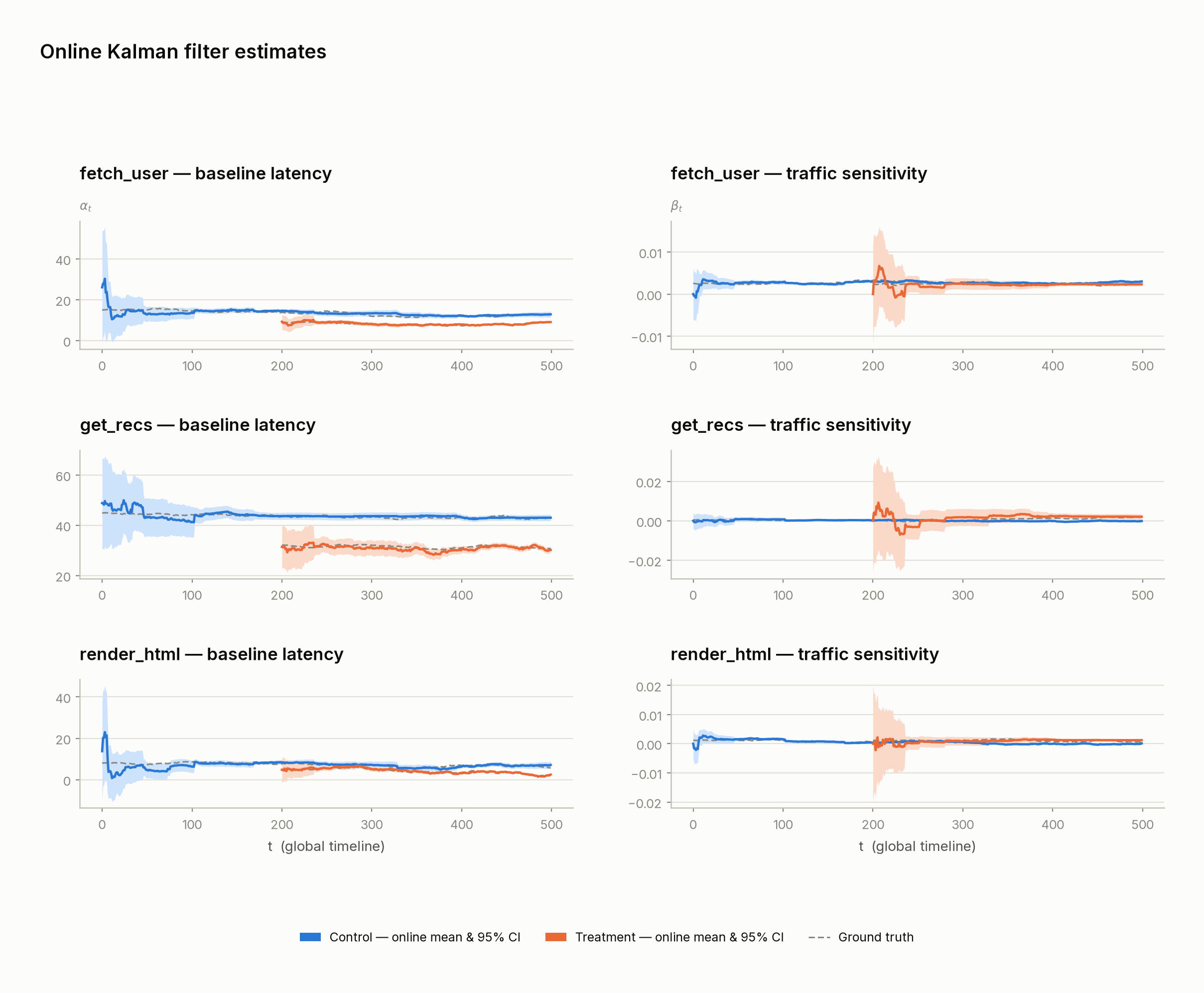
Two things worth noticing in that plot. First, the bands start wide and narrow as data accumulates — that's the filter being honest about not having enough information yet, not a bug. Second, the canary's bands stay visibly wider than control's throughout: less traffic means less information to pin down $\beta_t$, so its own numbers deserve less trust even when the posterior mean looks good. That's a real, useful signal, not an artifact to explain away.

Subtracting the fitted $\alpha_t + \beta_t \cdot \text{traffic}_t$ from the observed latency leaves a residual: the part of each function's latency traffic doesn't explain. That residual is what the rest of the pipeline works with.

Problem 2: a system is not a bag of independent metrics

Say you've done the above for all three functions and each one's residual mean looks a little better on treatment. Ship it? Not yet — because a system that passes three independent tests can still be more fragile as a system than the one it's replacing. If fetch_user gets slow, does get_recs still degrade gracefully, or does the whole chain slow down together now? Testing each function's latency in isolation can't answer that; it's a question about the joint distribution across functions, not any one function's marginal.

This is exactly what a copula is for. Sklar's theorem³ says any joint distribution factors into each variable's own marginal distribution plus a separate object — the copula — that captures only the dependence structure between them. Practically: rank-transform each function's residuals to a uniform margin (empirical CDF), push those through the inverse normal CDF, and take the Pearson correlation of the resulting normal scores. Because the transform strips out each variable's marginal shape, what's left is dependence — cleared of both traffic and of each function's own distributional quirks.

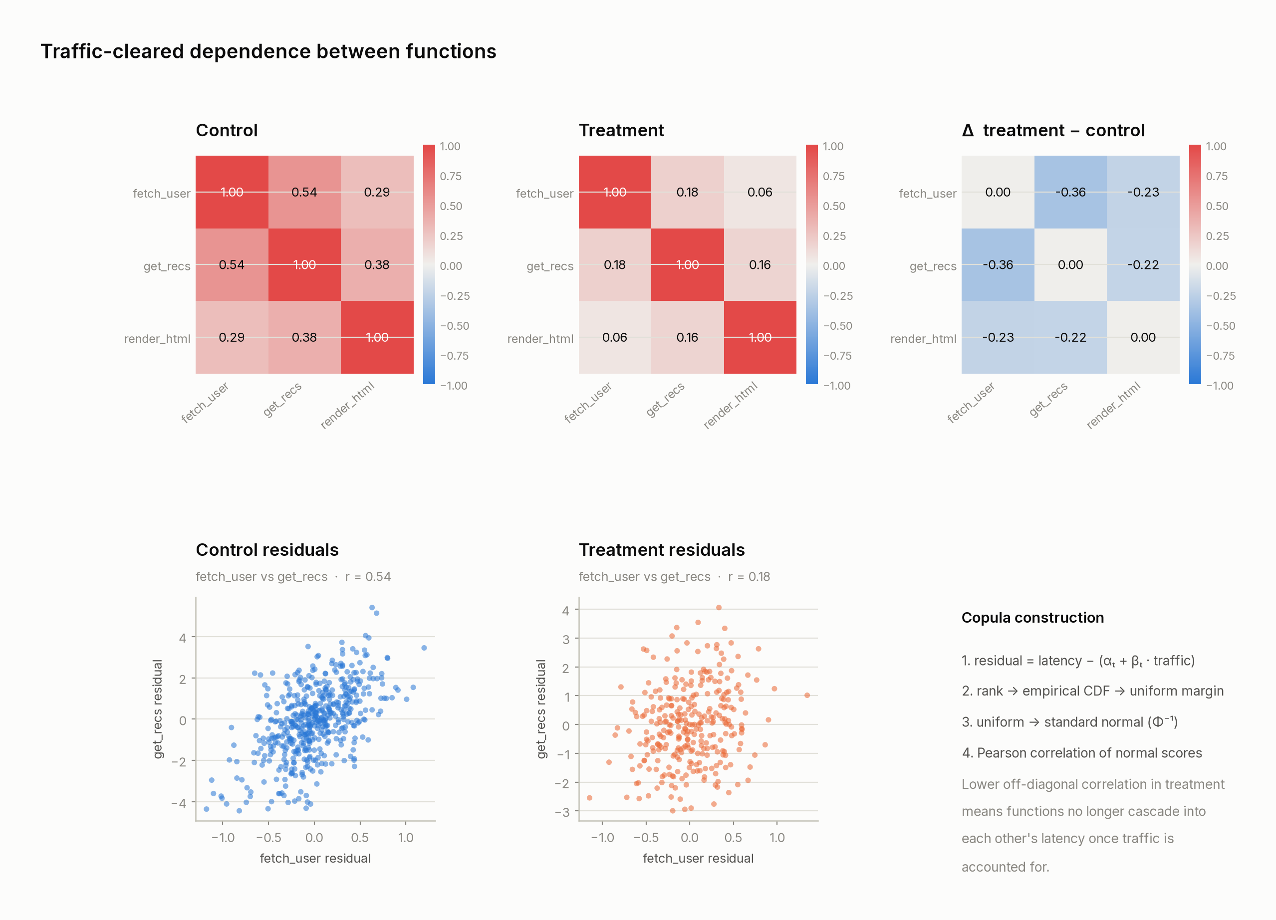
In control, fetch_user and get_recs residuals correlate at 0.54 — a slow database visibly drags recommendations down with it, even after removing what traffic explains. In treatment, that drops to 0.18. The new deploy isn't just faster on average, it's decoupled: a bad moment in one function is far less likely to cascade into the next one. That's a claim about system-level resilience a per-function latency comparison would never surface, because it isn't a statement about any single function's distribution — it's a statement about how they move together.

Problem 3: decide under uncertainty, at a shared reference point

Two more traps are easy to fall into even after fixing the first two. One: comparing arms at their own observed traffic rather than a common level — a canary at 10% share will look artificially fast if you don't equalize for load, which just reintroduces problem 1 through the back door. Two: eyeballing a mean difference on a dashboard and calling it a win, with no accounting for how confident that difference is.

The fix is to project both arms onto the same reference traffic level before comparing, and to turn the comparison into an explicit decision under uncertainty rather than a single point estimate: guardrails (mean latency must be lower, order 1; variance nice-to-have, order 2), Thompson sampling⁴ (draw one sample per arm per round, lower latency wins the round, tally $P(\text{arm is best})$), and the average treatment effect with its own credible interval.

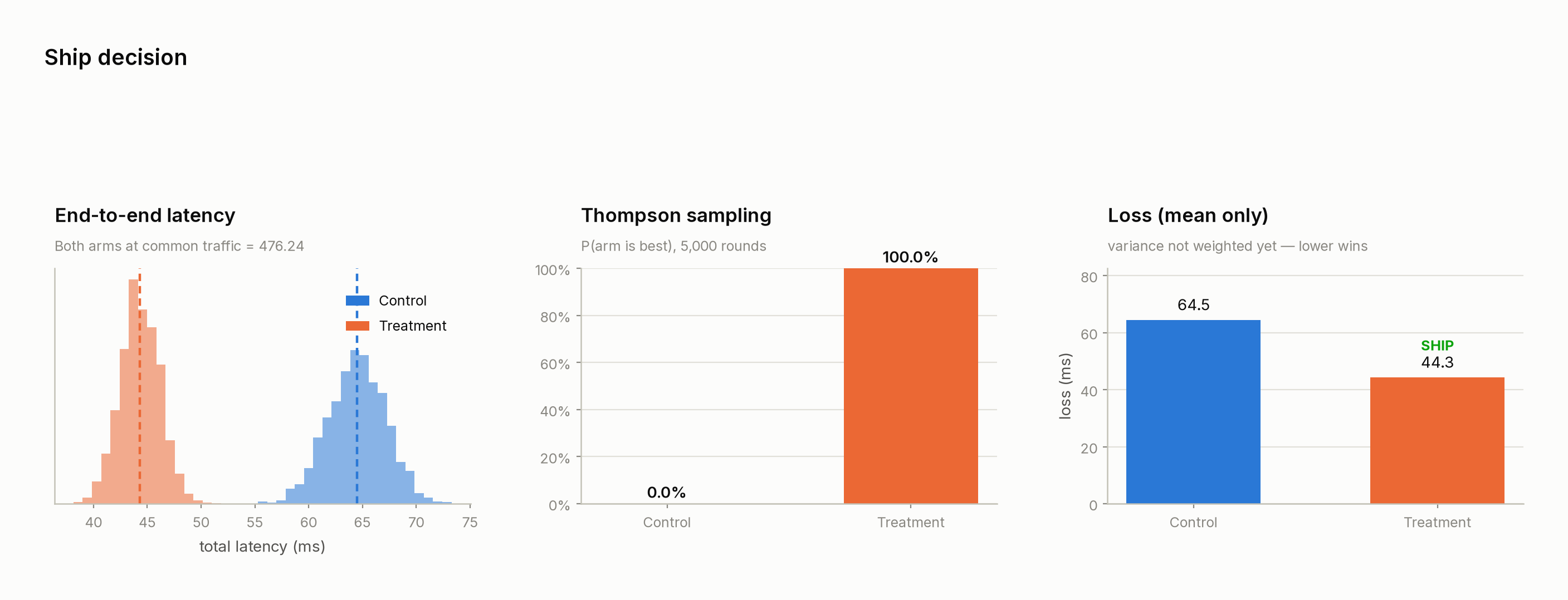
At a shared reference traffic level, treatment's whole-chain latency distribution sits cleanly to the left of control's — not because it's seeing less load, but because that confound has been projected out. Thompson sampling puts $P(\text{treatment is best}) = 100\%$ over 5,000 rounds, and the loss score picks treatment as the lower-risk arm. That's a ship decision made from the joint, traffic-adjusted, uncertainty-aware picture — not from a raw before/after average.

The three habits, generalized

None of this is specific to latency or to canaries. Testing a whole system rather than a metric comes down to three habits:

1. Model the environment before comparing outcomes. If the two things you're comparing didn't see the same conditions, the raw comparison is measuring the conditions as much as the thing you changed. Strip out what you can explain (here, traffic) before you compare what's left.
2. Test the dependency structure, not just each part. A system made of components that interact can regress as a system even when every component looks fine in isolation. If your components can cascade into each other, measure whether that coupling changed — not just whether each one's own average moved.
3. Decide under explicit uncertainty, at a shared reference point. A point estimate isn't a decision. Project both arms onto conditions they can be fairly compared at, then decide off a distribution — a win probability, a credible interval on the effect — not a single number that happens to look better today.

The repository has the full pipeline (src/kalman_filter.py, src/copula.py, src/scoring.py, src/run_ab_test.py) and a short academic writeup of the model with the full derivation. To point it at real telemetry instead of the simulation: feed simulate.py's output shape (t, deployment_id, arm, function_name, traffic, latency_ms) with your own per-function latency and traffic data, and run the Kalman fit + copula + scoring steps per arm.

References

Footnotes

1. M. West and J. Harrison. Bayesian Forecasting and Dynamic Models, 2nd ed. Springer, 1997. — the general dynamic linear model / Kalman filter framework used for the per-function traffic model. ↩

2. Online Mean and Variance Computations by Kalman Filtering. Unpublished note, 19 April 2026. — the scalar (no-regressor) case underlying the state and MLE equations; validated in tests/test_kalman_filter.py against the plain running mean and OLS in the relevant limits. ↩

3. A. Sklar. Fonctions de répartition à n dimensions et leurs marges. Publ. Inst. Statist. Univ. Paris, 8:229–231, 1959. — the theorem underlying the rank → empirical CDF → normal-scores copula construction in src/copula.py. ↩

4. W. R. Thompson. On the likelihood that one unknown probability exceeds another in view of the evidence of two samples. Biometrika, 25(3/4):285–294, 1933. — the sampling rule behind the win-probability score in src/scoring.py. ↩